Use a surrogate model to find the minimum of an expensive cost function

Sometimes our cost function can be expensive to compute, e.g. it may take 10 seconds to compute one value of our cost function and so calling it hundreds or thousands of times in an optimization may take hours.

One way to evaluate the minimum of an expensive cost function is to create a surrogate model. We can quickly evaluate the surrogate model, so we can call an optimization on the surrogate model to find its minimum. Then we can evaluate the the expensive cost function at that point and compare. This can result in a small number of calls to the cost function itself, but still find the minimum.

The key concepts you should gain from this page:

• How to create a surrogate model of an expensive cost function and use the surrogate model to guide the optimization.

An interpolated surrogate model

We start by defining a cost function like below. This should look familar from the previous section.

import numpy
from scipy import stats

def function(p):
    """ Executed for each set of drawn parameters in the optimization search.
    """

    # get the x and y values from Mystic
    x, y = p[0], p[1]

    # get value at Gaussian function x and y
    var = stats.multivariate_normal(mean=[0, 0], cov=[[0.5, 0],[0, 0.5]])
    gauss = -50.0 * var.pdf([x, y])

    # get value at volcano function x and y
    r = numpy.sqrt(x**2 + y**2)
    mu, sigma = 5.0, 1.0
    stat = 10.0 * (numpy.exp(-r / 35.0) + 1.0 /
                   (sigma * numpy.sqrt(2.0 * numpy.pi)) *
                    numpy.exp(-0.5 * ((r - mu) / sigma) ** 2)) + gauss

    # whether to flip sign of function
    # a positive lets you search for minimum
    # a negative lets you search for maximum
    stat *= 1.0

    return stat

Now we are going to use a WrapModel. This will take our cost function and create an archive for it.

We will sample for just a few points (e.g. 5) to create an initial surrogate model. We sample 5 points with truth.sample(bounds, pts=5) to initialize our surrogate model. You can change the truth.sample(bounds, pts=5) to truth.sample(bounds, pts=-5) to sample 5 points and run an optimization at each point. You should notice the number of data points in the surrogate model increase. Then we can use InterpModel to create the surrogate model.

We are going to create a while loop that goes until the error between our surrogate model and the optimization search reaches below a threshold. At each iteration of the while loop we are going to:

1. Update our surrogate model.

2. Find the minimum of the surrogate model.

3. Compute our cost function at that minimum.

4. Compare the value of the minimum at the surrogate and the cost function.

import os
import shutil
from spotlight.bridge.ouq_models import WrapModel
from spotlight.bridge.ouq_models import InterpModel
from mystic import tools
from mystic.solvers import diffev2
from mystic.math.legacydata import dataset, datapoint

# set random seed so we can reproduce results
tools.random_seed(0)

# remove prior cached results
if os.path.exists("volcano_surrogate"):
    shutil.rmtree("volcano_surrogate")

# generate a sampled dataset for the model
truth = WrapModel("volcano_surrogate", function, nx=2, ny=None, cached=False)
bounds = [(-9.5, 9.5), (-9.5, 9.5)]
data = truth.sample(bounds, pts=5)

# create surrogate model
surrogate = InterpModel("volcano_surrogate", nx=2, ny=None, data=truth, smooth=0.0, noise=0.0,
                        method="thin_plate", extrap=False)

# go until error < 1e-3
error = float("inf")
sign = 1.0
while error > 1e-3:

    # fit surrogate data
    surrogate.fit(data=data)

    # find minimum/maximum of surrogate
    results = diffev2(lambda x: sign * surrogate(x), bounds, npop=20,
                      bounds=bounds, gtol=500, full_output=True)

    # get minimum/maximum of actual expensive model
    xnew = results[0].tolist()
    ynew = truth(xnew)

    # compute error which is actual model value - surrogate model value
    ysur = results[1]
    error = abs(ynew - ysur)

    # print statements
    print("truth", xnew, ynew)
    print("surrogate", xnew, ysur)
    print("error", ynew - ysur, error)
    print("data", len(data))

    # add latest evaulated point with actual expensive model to be used by surrogate in fitting
    pt = datapoint(xnew, value=ynew)
    data.append(pt)

import pox
pox.rmtree("volcano_surrogate")

Warning: Maximum number of iterations has been exceeded
truth [9.499999999999948, 9.499999998663952] 6.812281772564118
surrogate [9.499999999999948, 9.499999998663952] -9.150964386952062
error 15.96324615951618 15.96324615951618
data 5
Warning: Maximum number of iterations has been exceeded
truth [-3.1699938681495423, 9.499999999999982] 7.511581413527667
surrogate [-3.1699938681495423, 9.499999999999982] -119.41260291584939
error 126.92418432937706 126.92418432937706
data 6
Warning: Maximum number of iterations has been exceeded
truth [-9.5, -9.499999999999993] 6.812281772380233
surrogate [-9.5, -9.499999999999993] -29.564642474061188
error 36.37692424644142 36.37692424644142
data 7
Warning: Maximum number of iterations has been exceeded
truth [0.00028208514725980044, -0.011770443619320524] -5.916635826059222
surrogate [0.00028208514725980044, -0.011770443619320524] -5.916230755309444
error -0.00040507074977824686 0.00040507074977824686
data 8

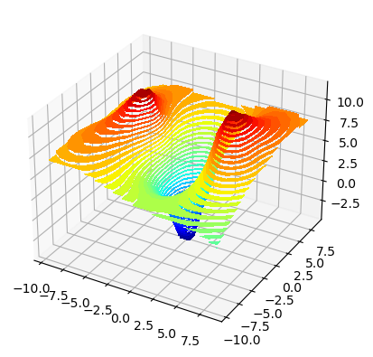
We can also plot the surface our surrogate model to see what it currently looks like.

import mystic
# show what our model currently looks like
mystic.model_plotter(lambda x: surrogate(x), depth=True, fill=True, bounds='-9.5:9.5,-9.5:9.5')

ML surrogate models

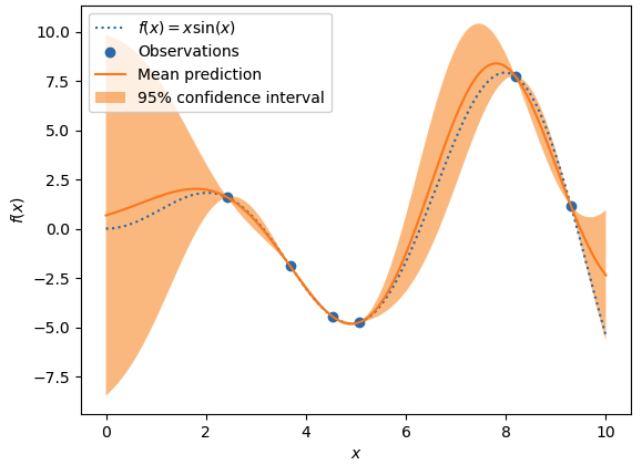
Instead of interpolating the surface, we can use a machine learning technique such as an artificial neural network (ANN) or a Gaussian process regressor (GPR). Below, we show an example of using a Gaussian process regressor to accomplish the same analysis. You can change method below to switch between the GPR and an ANN. We recommend using the GPR for this example.

To build a GPR we are going to use the scikit learn GaussianProcessorRegressor class. Illustration of a GPR on a 1D dataset is shown below.

from sklearn.gaussian_process import GaussianProcessRegressor as GPRegressor
from sklearn.gaussian_process.kernels import RBF, WhiteKernel
from sklearn.neural_network import MLPRegressor
from sklearn.preprocessing import StandardScaler
from spotlight.bridge.ml import Estimator, MLData, improve_score
from spotlight.bridge.ouq_models import LearnedModel

# set random seed so we can reproduce results
tools.random_seed(0)

# remove prior cached results
if os.path.exists("ml_surrogate"):
    shutil.rmtree("ml_surrogate")

# generate a sampled dataset for the model
truth = WrapModel("ml_surrogate", function, nx=2, ny=None, cached=False)
bounds = [(-9.5, 9.5), (-9.5, 9.5)]
data = truth.sample(bounds, pts=5)

# create surrogate model
method = "gp"
if method == "gp":

    # create our sklearn GPR
    kernel = RBF(length_scale=1.0, length_scale_bounds=(1e-05, 100000.0))
    regressor = GPRegressor(alpha=1e-10, optimizer=None, n_restarts_optimizer=0, kernel=kernel)

    # create our learned surrogate model in Mystic
    gpr = Estimator(estimator=regressor, transform=StandardScaler())
    best = improve_score(gpr, MLData(data.coords, data.coords, data.values, data.values), tries=10, verbose=True)
    surrogate = LearnedModel("ml_surrogate", nx=2, ny=None, data=truth,
                             estimator=best.estimator, transform=best.transform)

else:

    # create our sklearn multi-layer perceptron regressor
    regressor = MLPRegressor(hidden_layer_sizes=(100, 75, 50, 25),  max_iter=1000, n_iter_no_change=5, solver='lbfgs', learning_rate_init=0.001)

    # create our learned surrogate model in Mystic
    mlp = Estimator(estimator=regressor, transform=StandardScaler())
    best = improve_score(mlp, MLData(data.coords, data.coords, data.values, data.values), tries=10, verbose=True)
    surrogate = LearnedModel("surrogate", nx=2, ny=None, data=truth,
                             estimator=best.estimator, transform=best.transform)

# go until error < 1e-3
error = float("inf")
sign = 1.0
while error > 1e-3:

    # fit surrogate data
    surrogate.fit(data=data)

    # find minimum/maximum of surrogate
    args = dict(bounds=bounds, gtol=500, full_output=True)
    results = diffev2(lambda x: sign * surrogate(x), bounds, npop=20, **args)

    # get minimum/maximum of actual expensive model
    xnew = results[0].tolist()
    ynew = truth(xnew)

    # compute error which is actual model value - surrogate model value
    ysur = results[1]
    error = abs(ynew - ysur)

    # print statements
    print("truth", xnew, ynew)
    print("surrogate", xnew, ysur)
    print("error", ynew - ysur, error)
    print("data", len(data))

    # add latest evaulated point with actual expensive model to be used by surrogate in fitting
    pt = datapoint(xnew, value=ynew)
    data.append(pt)

import pox
pox.rmtree("ml_surrogate")

score = 1.0
score = 1.0
score = 1.0
score = 1.0
score = 1.0
score = 1.0
score = 1.0
score = 1.0
score = 1.0
score = 1.0
score = 1.0
score = 1.0
score = 1.0
reached max tries
no improvement
Warning: Maximum number of iterations has been exceeded
truth [1.4846419769916262e-07, -1.1220506456383777e-08] -5.915479484522285
surrogate [1.4846419769916262e-07, -1.1220506456383777e-08] -5.915479384931473
error -9.959081204158338e-08 9.959081204158338e-08
data 5

You should now have an understand how to implement an optimization search if the cost function is expensive to compute. We will now move on to how the topics we have covered on the prior pages can be implemented in a Rietveld analysis using MILK.

This tutorial is not meant as a comphrehensive tutorial on Mystic. For more Mystic documentation and examples, you can check out the Mystic Documentation.